Archive for the 'Back of the Envelope' Category

Morning-After Arithmetic

I take it that the following states are undecided:

Pennsylvania
Georgia
Michigan
North Carolina
Wisconsin
Nevada

By my calculations, this election is a tie if Trump wins (precisely) any of the following three subsets:

A = {Pennsylvania, Georgia, Michigan}
B = {Pennsylvania, Georgia, Wisconsin, Nevada}
C= {Pennsylvania, Michigan, Wisconsin, Nevada}

It is a Trump victory if Trump wins any of the following:

1) Any superset of A, B or C.
2) Any superset of {Michigan, Georgia, North Carolina, Wisconsin}
3) Any superset of {Michigan, Georgia, North Carolina, Nevada}

I went to bed believing that 98 – 47 = 41, and therefore had this all wrong, but I think it’s right now. Does anyone want to check my arithmetic?

Print Friendly, PDF & Email
Share

Take the Tablet

My thoughts on risk assessment and Covid-19 policy are here.

Click here to comment or read others’ comments.

Print Friendly, PDF & Email
Share

This is What a Pandemic Looks Like

woodstocksmall

This was Woodstock. As Jeffrey Tucker reminds us, Woodstock took place in the midst of a global pandemic that claimed more American lives than has Covid-19 (at least so far) — at a time when the population was much smaller . After correcting for population size and demographics, Tucker estimates the Hong Kong flu epidemic of 1969 killed the equivalent of 250,000 contemporary Americans, compared to under 100,000 so far for the current affliction.

Yet in 1969, American life went on pretty much as normal. As Tucker points out:

Stock markets didn’t crash because of the flu. Congress passed no legislation. The Federal Reserve did nothing. Not a single governor acted to enforce social distancing, curve flattening (even though hundreds of thousands of people were hospitalized), or banning of crowds. No mothers were arrested for taking their kids to other homes. No surfers were arrested. No daycares were shut even though there were more infant deaths with this virus than the one we are experiencing now. There were no suicides, no unemployment, no drug overdoses attributable to flu.

Media covered the pandemic but it never became a big issue.

The Woodstock producers flew in a dozen doctors to have on hand in case of a fast-spreading virus, but they seem to have given no serious thought to the prospect of cancelling.

Why such a difference between then and now? Tucker suggests a few possible culprits (the 24 hour news cycle, political and cultural shifts, etc.), but the first thing that came to my mind was that folks today are a whole lot richer than folks in 1969, and can therefore much better afford to take a few months off. If the average worker in 1969 had taken a four-month unscheduled vacation without any assistance, he’d have gone hungry — and the amount of available assistance was limited by the fact that everyone else was a lot poorer then too.

Here are the key facts we need to test that theory:

  • The income of the average American today is about two-and-a-half times what it was in 1969.
  • The income elasticity of the value of life is estimated to be somewhere between .5 and 1.0, and probably toward the lower end of that range for a developed country like the United States. I’ll take it to be .6. Here the “value of life” refers to the amount people are willing to pay to avoid a given small chance of death, and the elasticity estimate means that the value of your life is (approximately) proportional to I.6, where I is your income.

Taken together, these facts imply that the value of a life in 1969 was about 58% of what it is today, which in turn implies that people would have been willing to put up with only 58% as much lost income in exchange for the same amount of safety. If you’re willing to tolerate six months without a paycheck to avoid, say, a 1% chance of death, then your 1969 self would have been willing to tolerate only about three-and-a-half months. If avoiding that 1% chance of death requires, say, a five-month lockdown (or any other length longer than three-and-a-half months but shorter than six), then you’re going to favor that lockdown, though you’d have scoffed at the thought of it in 1969.

Even this fails to account for another factor: A national shutdown of a given length would have been a lot costlier in 1969 than it is in 2020, when a good 30% of us can work from home. Perhaps a six-month lockdown only costs us (on average), say, three month’s income. (I pulled that “three months” out of my hat. I’m sure with a little research I could have done better.) If that’s what we’re willing to tolerate for a given amount of safety, then our 1969 selves would have tolerated only a one-and-three-quarter months’s income loss, which might have meant something like a two month lockdown. Where we’d tolerate six months, they’d tolerate only two.

In other words: Nobody considered locking down the economy in 1969 because they couldn’t afford to (or more precisely, given their relative poverty, they preferred to spend their wealth on other things). Today’s lockdown is widely supported because it’s a luxury we’ve grown rich enough to afford. In other words, the lockdown is yet another triumph of capitalism.

That, at least, is what the back of my envelope says. I expect there are people who have thought about this a whole lot harder than I have. I hope we hear from some of them.

Print Friendly, PDF & Email
Share

The Value of Life — What’s Wrong With This Picture?

Trapeze Artist

Edited to add: As Salim suggests in comments, the entire problem is that I assumed an implausible value for wealth (which should be interpreted as lifetime consumption). With a more plausible number, everything makes sense. Mea culpa for not realizing this right away. I will leave this post up as a monument to my rashness, but have inserted boldfaced comments in appropriate places to update for my new understanding.

This is bugging me. It’s a perfectly simple exercise in valuing lives for the purposes of cost-benefit analysis. I would not hesitate to assign it to my undergraduates. But it leads me to a very unsettling and unexpected place, and I want to know how to avoid that place.

It’s also a little geeky, so I hope someone geeky will answer — ideally, someone geeky who thinks about this stuff for a living.

Start here: You’re a trapeze artist who currently works without a net. There’s a small probability p that you’ll fall someday, and if you fall you’ll die. You have the opportunity to buy a net that is sure to save you. What are you willing to pay for that net?

Well, let’s take U to be your utility function and W your existing wealth. If you don’t buy the net, your expected utility is

p U(death)+(1-p) U(W)

But we can simplify this by adding a constant to your utility function so that U(death)=0. So if you don’t buy the net, your expected utility is just

(1-p )U(W)

If you do buy a net at price C, then you’re sure to live, with utility

U(W-C) = U(W) – C U′ (W)

where the equal sign means “approximately equal” and the approximation is justified by the assumption that the probability of falling (p) is small, so your willingness to pay (C) is presumably also small.

Equating these two expected utilities gives me C = p U(W)/U′ (W). If we set V = U(W)/U′ (W), then C = pV. That is, you’re willing to pay pV to protect yourself from a p-chance of death. This justifies calling V the “value of your life” and using this value in cost-benefit calculatios regarding public projects that have some small chance of saving your life (guard rails, fire protection, etc.)

So far, so good, I think. But now let’s see what happens when we posit a particular utility function.

I will posit U(W) = log (W), which is a perfectly standard choice for this sort of toy exercise, though actual real-world people are probably a bit more risk-averse than this. Except I can’t just leave it at U(W) = log(W), because my analysis requires me to add some constant T to make the utility of death equal to zero.

So let’s take E to be the income-equivalent of death; that is, living with E dollars is exactly as attractive as not living at all. Then I have to choose T so that log(E) + T = 0. In other words, T = -log(E).

Now I know that, with your current wealth equal to W, the value of your life is U(W)/U'(W) = W log(W/E) .

Now as a youngish but promising trapeze artist, you’ve probably got some modest savings, so lets make your current wealth W=50,000 (with everything measured in dollars). (Edited to add: This was the source of all the difficulty. W represents something like lifetime consumption, so 50,000 is a ridiculously small number. Let’s go with 5 million instead.) Then here is the value of your life, as a function of E, the income-equivalent of death.

If E = .0001 (that is, if dying seems just as attractive to you as living with your wealth equal one-one-hundredth of a penny), then the value of your life is $1 million. (Edited to add: This should actually be E= 4.1 million dollars, which is considerably more than one-one-hundredth of a penny.)

If E = 6.92 x 10-82, then the value of your life is $10 million. (Edited to add: This should be E = $677,000 which might be a plausible figure.)

If E = 1.29 x 10-864, then the value of your life is $100 million. (Edited to add: This should be E equal to about one cent, which is of course implausible, but that’s fine, because a $100 million value of life is also implausible.)

Edited to add: I won’t continue to edit the details in the rest of this post, but I think this is all straightened out now. Thanks to those who chimed in, and sorry to have taken your time on this!

Now I am extremely skeptical that you, I, or anyone else is capable of envisioning the difference between living on 10-82 dollars and living on 10-864 dollars. Yet the decision of whether to value your life at $10 million or at $100 million hinges entirely on which of these seems more to you to be the utility-equivalent of death.

There is some purely theoretical level at which this is no problem. It is possible that you’d rather die than live on 10-864 dollars and would rather live on 10-863 dollars than die. But I am extremely skeptical of any real-world cost-benefit analysis that hinges on this distinction.

(And this is the range in which we have to be worried, since empirical estimates of the value of life tend to come in somewhere around $10 million.)

If I make you less risk-averse — say with a relative risk aversion coefficient of 4 — almost the entire problem disappears. But the tiny part that remains is still plenty disturbing. Then I get:

If E = .007 (that is, about 2/3 of a penny), the value of your life is $1 million.

If E = .003 (about 1/3 of a penny), your life is worth $10 million.

If E = .0015 (a sixth of a penny), your life is worth $100 million.

So we need to tell the folks in accounting to value your life at either $1 million or $100 million, depending on where you draw the suicide line between having two thirds of a penny and having one sixth of a penny.

This is nuts, right? And how squeamish should it make me about the whole value-of-life literature? And what, if anything, am I missing?

Click here to comment or read others’ comments.

Print Friendly, PDF & Email
Share

The Prestige Cost of Affirmative Action

I. The Issue

It’s often claimed (at least by politicians, journalists and their ilk) that affirmative action tends to “stigmatize” succcessful members of the favored group, in the sense that a Harvard professorship is less prestigious when it’s held by someone who might not have made it to Harvard without an affirmative action boost.

It’s approximately equally often claimed that this is effect is too small to worry about.

I’m not aware of anyone on either side of this argument having attempted to settle the question with arithmetic.

In their defense, the question can’t be settled by arithmetic, because it’s pretty hard to quantify the difference in “prestige” between a professorship that reveals you’re likely to be in the top one-one-hundredth of one percent of the population and a professorship that only reveals you’re likely to be in the top two-one-hundredths of one percent of the population. But we can at least give some answers contingent on different assumptions about this issue. (And contingent also, of course, on various modeling assumptions.)

II. A Model

To that end, here is a primitive first-pass model:

Continue reading ‘The Prestige Cost of Affirmative Action’

Print Friendly, PDF & Email
Share

Oxycontin: Yea or Nay

Should oxycontin be legal? Here’s what the back of my envelope says:

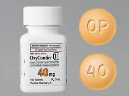
oxycontinIn the U.S., there are about 50 million prescriptions a year for oxycontin, most of them legitimate and for the purpose of alleviating severe pain. I’m going to take a stab in the dark and guess that the average prescription is for a two-week supply.

There are also (at least if you believe what’s on the Internet) about 20,000 deaths a year in the U.S. related to oxycontin abuse. If we value a life at $10,000,000 (which is a standard estimate based on observed willingness-to-pay for life-preserving safety measures), that’s a cost of 200 billion dollars a year, or $4000 per prescription.

If those were all the costs and benefits, the conclusion would be that oxycontin should be legal if (and only if) the average American is willing to pay $4000 to avoid two weeks of severe pain. I’m guessing that might be true in some cases (particularly when the pain is excruciating) but not on average. So by that (incomplete) reckoning, oxycontin should either be off the market entirely or regulated in some entirely new way that will dramatically reduce those overdose deaths.

But of course what this overlooks on the benefit side is all the “abusers” whose lives have been enriched by oxycontin. This includes the vast majority who use and live to tell the tale, and also some of the OD’ers, for whom a few years of oxycontin highs might well have been preferable to a longer lifetime with no highs at all. Relatedly, what this overlooks on the cost side is that the average “abuser” is likely to value his life at considerably less than the typical $10 million — as evidenced by the fact that he’s electing to take these risks in the first place. Also relatedly, it overlooks the likelihood that many of those who overdose on oxycontin would, in its absence, be killing themselves some other way.

If the back of your envelope is larger than mine and you make those corrections, I’m reasonably confident that your bottom line will come out pro-oxycontin. (Please share that bottom line!) I am however, mildly surprised (and — both as a blogger who prefers slam-dunk arguments and as a libertarian who prefers to come down on the side of freedom — mildly disappointed) that the first quick-and-dirty calculation comes out the other way.

Print Friendly, PDF & Email
Share

Is American Airlines too Reckless?

aa

My return trip from Lubbock to Rochester took almost 36 hours, due to maintenance issues on three separate aircraft. This leads me to wonder whether American Airlines is erring too far in the direction of safety and too little in the direction of getting people where they want to go — perhaps even recklessly so.

Here’s what the back of my envelope shows:

Continue reading ‘Is American Airlines too Reckless?’

Print Friendly, PDF & Email
Share

How Many Deaths Does It Take Till He Knows….?

President Trump wants to impose a 20% tariff on Mexican imports. How many Americans will that kill? Let’s play with some numbers.

The Bureau of Labor Statistics reports (I’m looking at Table 13 in that link) that in 2012, approximately 125 million U.S. households spent an average of $731 on fruits and vegetables. That’s about $91 billion altogether.

I learn from this page that the US imports about $9 billion worth of fresh fruits and vegetables each year from Mexico. That is, then, about 10% of our fruit and vegetable consumption.

I learn from various research reports around the web that the price elasticity of demand for fruits and vegetables is somewhere in the vicinity of .50. (Some say higher, some say lower). This means that a 20% tariff — as the president has just called for — will reduce imports by about 10%.

So the Trump tariff should reduce total U.S. fruit and vegetable consumption by about 10% of 10% — that is, about 1%.

(This is, deliberately, a considerable underestimate, since it entirely ignores the fact that the tariff will also lead to increases in the price of American vegetables, leading to further reduced consumption.)

Now here I learn that low fruit and vegetable consumption is associated with a higher risk of degenerative diseases, including cancer, cardiovascular disease, cataracts and brain dysfunction. “More than 200 studies in the epidemiological literature show, with great consistency, an association between low consumption of fruits and vegetables and high cancer incidence.” Many of the mechanisms for this are well understood. For example, folic acid deficiency leads to chromosome breaks and then to cancer. Your health risks do not drop off continuously with your vegetable consumption; instead there are sudden changes — you’re either above or below the level where chromosome breaks occur. (There are similar issues with at least eight other micronutrients — in addition to folic acid — that we get from fruits and vegetables.) About 10% of the U.S. population is below that critical level. Most of those have very low incomes. (The World Health Organization estimates that worldwide, about 5 million people a year die from inadequate fruit and vegetable consumption, and most of those are very poor.) For a first (very rough) approximation, let’s assume that those with folic acid deficiencies are in fact the poorest 10%. You can see here that these are people with individual incomes below about $10,000.

Continue reading ‘How Many Deaths Does It Take Till He Knows….?’

Print Friendly, PDF & Email
Share

How to Be Reasonable

Listening to Season One of NPR’s podcast Serial, which is the story of a real-life murder case, I came away about 80% sure that the defendant was guilty and 100% sure that I’d vote to convict him. This got me to pondering whether my standards for reasonable doubt (apparently less than 80% in this case) are in fact reasonable.

So I wrote down the simplest model I could think of — a model too simple to give useful numerical cutoffs, but still a starting point — and I learned something surprising. Namely (at least in this very simple model), the harsher the prospective punishment, the laxer you should be about reasonable doubt. Or to say this another way: When the penalty is a year in jail, you should vote to convict only when the evidence is very strong. When the penalty is 50 years, you should vote to convict even when it’s pretty weak.

(The standard here for what you “should” do is this: When you lower your standards, you increase the chance that Mr. or Ms. Average will be convicted of a crime, and lower the chance that the same Mr. or Ms. Average will become a crime victim. The right standard is the one that balances those risks in the way that Mr. or Ms. Average finds the least distasteful.)

Here (I think) is what’s going on: A weak penalty has very little deterrent effect — so little that it’s not worth convicting an innocent person over. But a strong penalty can have such a large deterrent effect that it’s worth tolerating a lot of false convictions to get a few true ones.

In case I’ve made any mistakes (and it wouldn’t be the first time), you can check this for yourself. (Trigger warning: This might get slightly geeky.) I assumed each crime has a fixed cost C to the victim and a random benefit B to the perpetrator. For concreteness, we can take C=2 and take Log(B) to be a standard normal distribution, though the results are pretty robust to these particulars. (Or, much more simply and probably more sensibly, take B to be uniformly distributed from 0 to C — the qualitative results are unchanged by this.)

Continue reading ‘How to Be Reasonable’

Print Friendly, PDF & Email
Share

The Ashley Madison Test of College Faculty Cluelessness

Science marches on. Recent developments have made it possible to answer the age-old question: What percentage of your college faculty used their work email addresses to establish accounts at Ashley Madison?

In a sample of 33 highly ranked colleges, the answer ranges from a low of 1.6% at Oberlin to a pretty much unbelievable 22.6% at the University of Minnesota. (The full rankings appear at the bottom of this post.)

I got these percentages by counting the number of unique email addresses ending with, say, “harvard.edu” in the leaked Ashley Madison database, and dividing by the number of Harvard faculty, as reported by the college either on its website or in its Common Data Set filings.

The methodology, is, of course, fraught with peril. First, the majority of academic email addresses belong not to faculty, but to students. But it seems like a good guess that faculty (by virtue of their average age) are both far more likely than students to be trolling Ashley Madison, and far more likely than students to be clueless about acquiring anonymous email addresses. Besides, a quick spotcheck of the email addresses in the Ashley Madison database does indeed confirm that most of them (at least in one small but random sample) belong to faculty members.

There are also, of course, staff, and the staff-to-faculty ratio probably varies a lot from school to school, so weeding out the staff could change the relative rankings quite a bit. But again, my (still small but still random) sample continues to indicate that these are mostly faculty members.

A far more important issue might arise from the fact that some universities have multiple campuses. It’s possible, for example, that the 657 umn.edu email addresses in Minnesota’s numerator came from many campuses, while the 2913 facuty in their denominator represents only the main campus. This will tend to inflate the rankings of the big state schools, and might account for the appearance of Minnesota, Virginia, Michigan and Cornell at the top — suggesting that if the numbers were crunched more carefully, the prize might go to Liberty University. If I were going to use these rankings for anything important, I’d give this issue a harder look.

One might also note that anybody can type anybody else’s email address into Ashley Madison, but I’m inclined to discount the importance of that, because it’s hard for me to see what the motive would be (except, perhaps, as part of a campaign to flood someone’s email box with unwanted replies).

With those caveats, feel free to use these rankings as a measure of your college faculty’s average cluelessness, at least when it comes to maintaining anonymity over the Internet.

Continue reading ‘The Ashley Madison Test of College Faculty Cluelessness’

Print Friendly, PDF & Email
Share

Veterans Affairs

Suppose you’ve just joined the army and expect to serve for, oh, say, four years before returning to civilian life.

Which would you rather have when you get out: a lifetime-guaranteed annual check for $7500 (adjusted each year for inflation) or a package of VA benefits?

To help you decide: The VA benefits include payments of anywhere from about $100 a month to almost $3000 a month in the unlikely event that you are partially or fully disabled, a pension on the order of $15,000 a year in the more unlikely event that you are both disabled and poverty-stricken (rising to more like $20,000 a year if you need regular aid and attendance), educational benefits under the GI bill, and health care of whatever quality the government chooses to provide.

Me, I’d take the guaranteed $7500-a-year in a heartbeat. If that’s the typical response, then it’s hard to see why we have a Veteran’s Administration in the first place, seeing as how the VA’s annual budget would just about cover those payments.

Continue reading ‘Veterans Affairs’

Print Friendly, PDF & Email
Share

High Frequency Rentseeking

Spread Networks recently spent $300 million to build a fiberoptic cable that will let Wall Street traders shave .003 seconds off their execution times.

What’s the social value of that cable? If you can shave .003 seconds off the time it takes to execute a trade, how much good have you done the world?

Clearly, the full value of the cable resides in its ability to get things done faster. So start with a vast overestimate: Suppose the entire economy is on hold waiting for that trade to be completed. Then, thanks to the cable, we can all get on with our lives .003 seconds sooner and produce an extra .003 seconds worth of output.

In a $15-trillion-a-year economy, that comes to about $1500.

If we assume, more realistically, that just 1/1000 of the economy is hanging fire waiting for this one trade, the social contribution of a .003-second speedup is roughly $1.50. I’m confident it’s even more realistic to replace that 1/1000 with 1/1,000,000 . That gets us down to about an eighth of a cent.

But chances are you’d be willing to pay a hell of a lot more than an eighth of a cent for that extra speed, which is why Spread Networks is willing to pour $300 million into this thing, and why, quite generally, we should expect there to be more invested in such projects than they return in social value.

Continue reading ‘High Frequency Rentseeking’

Print Friendly, PDF & Email
Share

The Arithmetic of Wage Gaps

Mark Perry and Andrew Biggs argue in the Wall Street Journal that

These gender-disparity claims [the claims that women are paid 23% less than men for the same work] are also economically illogical. If women were paid 77 cents on the dollar, a profit-oriented firm could dramatically cut labor costs by replacing male employees with females. Progressives assume that businesses nickel-and-dime suppliers, customers, consultants, anyone with whom they come into contact — yet ignore a great opportunity to reduce wages by 23% [by hiring women instead of men].

Well, first of all, even if we take the gender disparity claims at face value, this doesn’t add up to an opportunity to reduce wages by 23%. Only about half the work force is female, so the average firm, if it replaced all of its men with women earning 23% less, would reduce its wage bill by only about 11.5%.

Beyond that, the Perry/Biggs argument appears to founder on the observation that lazy and incompetent managers do in fact manage to ignore profit opportunities all the time. Why, then, is it so hard to imagine that they’re ignoring this one?

Fortunately, I’m here to fill the gap —- by figuring out just how big a profit opportunity we’re talking about.

Continue reading ‘The Arithmetic of Wage Gaps’

Print Friendly, PDF & Email
Share

MegaOdds

In case you’re thinking of running out for a MegaMillions lottery ticket in the few hours left before tonight’s drawing: If you drive one mile to buy your ticket, your chance of being involved in a fatal accident on the way is about 8 times as great as your chance of winning the jackpot.

Click here to comment or read others’ comments.

Print Friendly, PDF & Email
Share

Aaagh!

I am buying a house, and am therefore faced with the choice between a 15 year mortgage at 2.875% and a 30 year mortgage at 3.49% (as of a couple of days ago; those rates have probably changed a little by now).

The main advantage of the 15 year mortgage is that it comes with a lower interest rate and, because I’m making larger monthly payments, it keeps my money out of the stock market, which is good if the market tanks. The main advantage of the 30 year mortgage is that it allows me to keep more money in the stock market for a much longer time, which is good if the market does well.

How should I weigh those factors? Economics tells me that I will solve this problem by forecasting the return on equities over each of the next 30 years, and computing, on the basis of my forecast, which mortgage will leave me richer in the long run. No, that’s not quite right. Actually, economics tells me that I’ll make many forecasts, assign each one a probability, and thereby compute two probability distributions for my future net worth and then choose the distribution I prefer.

Now let’s get serious.

Continue reading ‘Aaagh!’

Print Friendly, PDF & Email
Share

Charting the Tax Plans

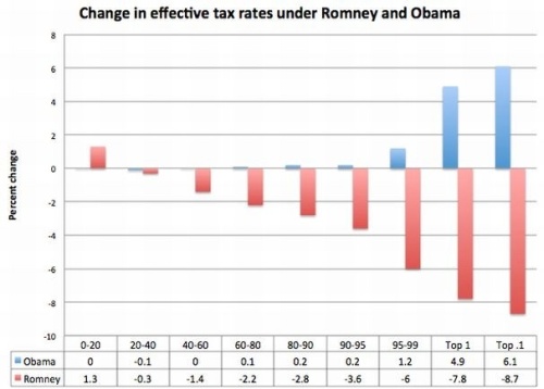
Ezra Klein, quoted with approval by Paul Krugman, offers this chart of how the Obama and Romney tax proposals will change rates for taxpayers in various quintiles:

What we’re supposed to infer, according to Krugman, is that

we have an election in which one candidate is proposing a redistribution from the top … downward, mainly to lower-income workers, while the other is proposing a large redistribution from the poor and the middle class to the top.

But no such thing is remotely true. What we actually have is an election in which both candidates are proposing massive redistributions from the top downward, one slightly less so than the other. You’d never know this from looking at Klein’s chart because it illustrates changes in rates, whereas what actually matters is the rates themselves. It makes no sense to ask whether any particular group ought to be paying more or less without reference to how much they’re already paying.

Indeed, this is a classic example of what I once called the “Grandfather Fallacy” — by focusing on changes instead of absolutes, Klein’s chart conceals any existing inequities and hence treats them as “grandfathered in”.

Fortunately, Greg Mankiw has provided the numbers that allow us to make the requisite correction. Here, according to Mankiw, are the current tax burdens on various income groups (counting transfers as negative taxes, as of course one should):

Bottom quintile: -301 percent
Second quintile: -42 percent
Middle quintile: -5 percent
Fourth quintile: 10 percent
Highest quintile: 22 percent

Top one percent: 28 percent

That “-301 percent” means, for example, that a typical family in the bottom quintile receives $3.01 in net transfers for every $1 that it earns.

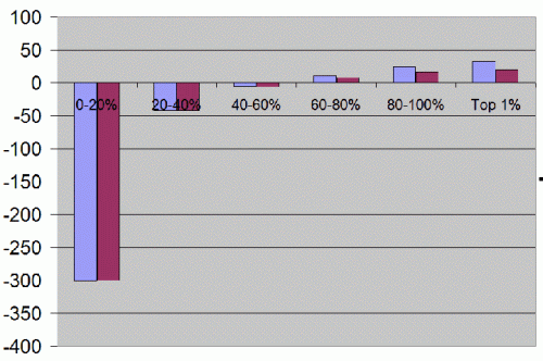
By adding these numbers to the numbers in Klein’s graph, we can construct a picture that actually depicts something interesting, namely the projected tax burdens for each group. It looks like this (the vertical axis represents percentage of income):

Note, for example, that, contrary to the impression you might have gotten from Klein’s and Krugman’s posts, both plans place the highest percentage burden on the top 1%, and both plans place a negative burden on the middle quintile — though Obama’s does both of these things to an ever-so-slightly greater extent than Romney’s does. There’s room for disagreement about which plan is fairer, but no room, I think, for disagreement about which chart is relevant.

Continue reading ‘Charting the Tax Plans’

Print Friendly, PDF & Email
Share

Lifeboats on the Titanic

titanicShould RMS Titanic have carried more lifeboats? Yes, probably. But it took me a few minutes to convince myself.

Roughly 1500 died on the Titanic; according to Wikipedia, it would have cost about $16,000 to equip her with additional lifeboats sufficient to save them all. Call it $10 per life saved. The price level today is roughly 22 times what it was in 1912, so in today’s terms that’s $220 per life.

Now, if I were boarding a ship for a luxury cruise, and was offered the chance to pay an additional $220 for a guaranteed seat on a lifeboat in the event of a sinking, I’m quite sure I’d take a pass — and I’m quite sure so would virtually all of my fellow passengers. So if the Titanic had been designed to cross the ocean once and then spend the rest of its days in a museum, it would have been insane to equip her with extra lifeboats. But of course if the Titanic had been designed to cross the ocean once and then spend the rest of its days in a museum, it would have been insane to build her in the first place. So that’s not the right calculation.

The right calculation accounts for the fact that a single lifeboat provides security to passengers on multiple voyages. How many voyages? Well, the Titanic was intended to make the round trip between Europe and America every three weeks; that’s two voyages per three-week period. I’m not sure how long the sailing season was, but we know it was underway by mid-April (and perhaps earlier; it’s often mentioned that if the Titanic had been ready earlier she would have sailed earlier) so (assuming sailing conditions are roughly symmetric around the solstice) it must have lasted till at least mid-August. That’s time for five round trips at a minimum, and I’m guessing this is a quite conservative assumption.

If a lifeboat lasts a year, then, it does its job at least ten times. If it lasts five years (which is, I suspect, another quite conservative assumption), it does its job fifty times. Now we’re in the vicinity of $4 per passenger (and of course much less if my assumptions are indeed quite conservative).

Continue reading ‘Lifeboats on the Titanic’

Print Friendly, PDF & Email
Share

Women’s Wages and the Back of My Envelope

Yesterday’s breathtakingly dishonest graph from the AFL-CIO touched off some discussion in comments about whether the male/female wage differential could plausibly be driven by employer discrimination.

The usual argument to the contrary runs like this: If the differential is driven by employer discrimination (as opposed to, say, the abilities and/or preferences of the workers), then non-discriminating employers (i.e. those who care only about making a buck, regardless of who they have to hire to do it) would draw only from the relatively cheap female labor pool. It wouldn’t take many of these non-discriminating employers to drive women’s wages up to the same level as men’s. We don’t see that happening, ergo the hypothesis of employer discrimination is refuted.

The problem with that argument is that it assumes employers won’t ignore a profit opportunity, whereas in fact employers ignore profit opportunities all the time — by keeping on their incompetent nephews, taking Wednesday afternoons off to play golf, or, yes, hiring people they like having around instead of people who could do a better job.

Continue reading ‘Women’s Wages and the Back of My Envelope’

Print Friendly, PDF & Email
Share